The Heights of Folly
I won’t say I’m a great fan of clear cutting but I suppose some may find this image inspiring (from a recent walk to the Sign of the Packhorse). We start with this as it will later help to illustrate some of the analysis the GIS courses have been doing lately. We’ve been spending a bit of time with LiDAR data; more specifically, we’ve been looking at how to use data like these to determine the amount of tree cover within a given area, along the lines of what the Auckland Council did a few years ago with mapping the urban forest in the Waitemata Local Board area, an example of which is shown below:
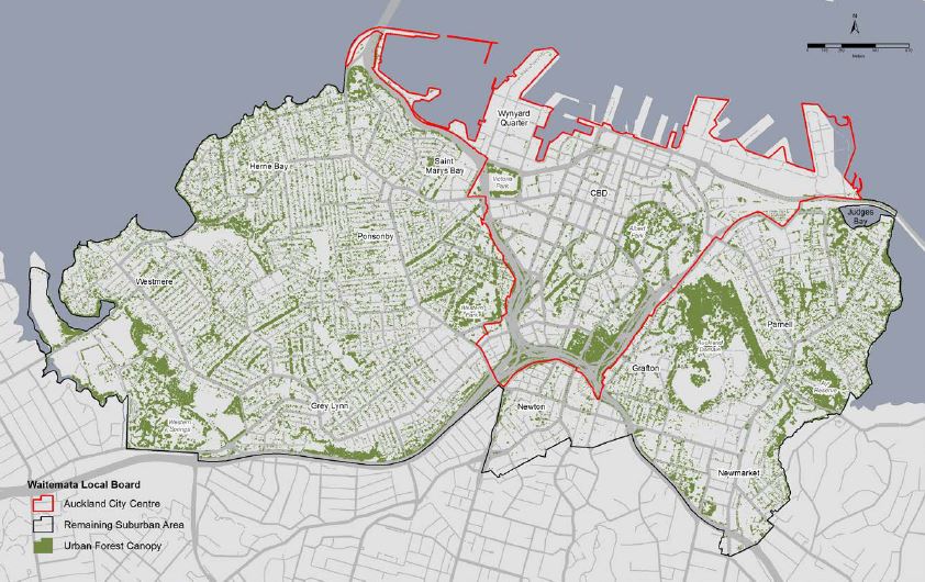
Here they’ve used LiDAR data to map vegetation greater than 3 m in height at high resolution, down to individual trees in some cases. We aimed to recreate this analysis for various places across the motu.
As you may recall, LiDAR data give us high-resolution elevation data as a cloud of points, with these points often spaced around 0.5 m apart across large areas. These data have transformed a lot of what we can do analysis-wise, and this is just one small taste of it. While the main benefit of LiDAR is elevation, depending on how the data are processed, we can also identify specific types of features on the ground. Amongst the wide variety of possible codes, points can be classified into things like vegetation, buildings, road surfaces and even transmission towers and wires. As an example, we’ll look at a data set captured in over 2020 and 2021 over the area shown below:
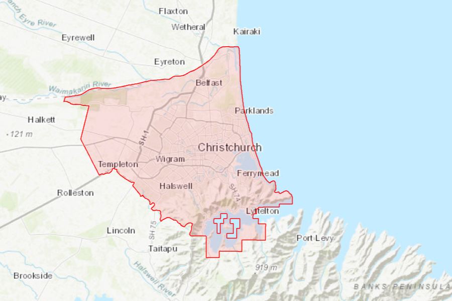
This dataset has a limited number of classification codes, but the ones available are quite pertinent to our analysis:
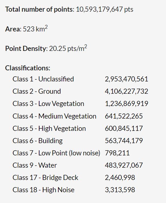
We can use the Low, Medium and High Vegetation points to map out where the vegetation is and how tall it is. For this post, I thought I’d show how this can be done for Quail Island:
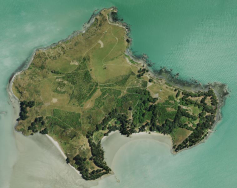
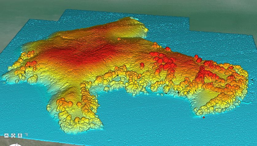
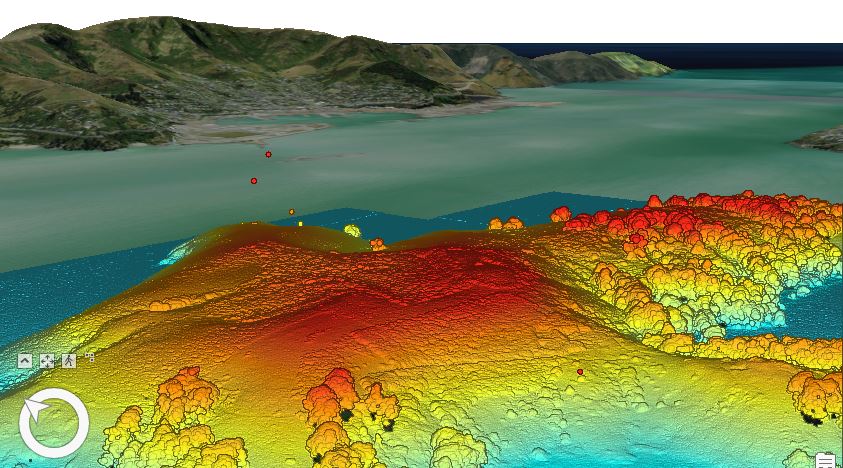
Of course I’m not going to need all 10+ billion points for just Quail Island. From the OpenTopography site I can crop out what I need and download the raw LiDAR point cloud for use in Pro. Even with that, I end up with 35+ million. Shown in 3D, my LiDAR points are clearly picking out trees and surface features as well as areas of open grassland:
With these points, I’ve got high-precision locations with x, y and z coordinates – a very important facet is that the elevations are all with respect to mean sea level (and we know how fraught that can be). We can use the LiDAR data to create two elevation models: a Digital Elevation Model (DEM) which has the bare earth elevations, i.e. the ground with no features (trees, buildings, etc) and the Digital Surface Model (DSM) which includes the tops of trees and buildings and anything else above ground level. To put that in the context of our analysis, let’s return to the clear cut image above.
Below, the white line at the base of the trees shows us a profile of the bare earth DEM while the blue line shows the profile along the DSM – the tops of the trees. Clearly, most of these trees are around the same height, but the elevation of the tops of the trees (above sea level) depends on where on the landscape they are. We need to take this into account somehow.
What we get from the LiDAR data are the DEM and DSM elevations above sea level. So,
Actual Tree Height = DSM Elevation – DEM Elevation
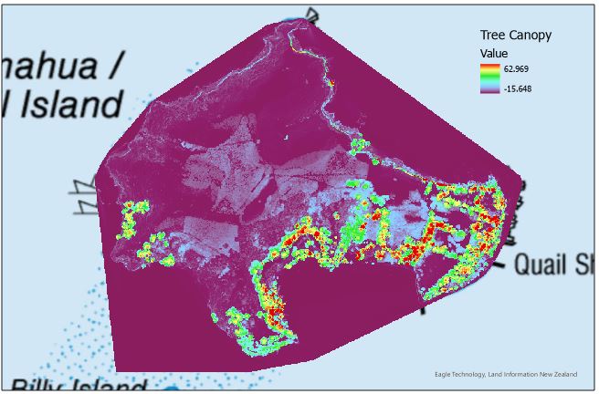
This ends up being pretty easy once we’ve created our respective DEMs and DSMs – it’s just a quick raster calculation. Then we know the height of any vegetation at each grid cell. For Quail Island, my result looked something like this:
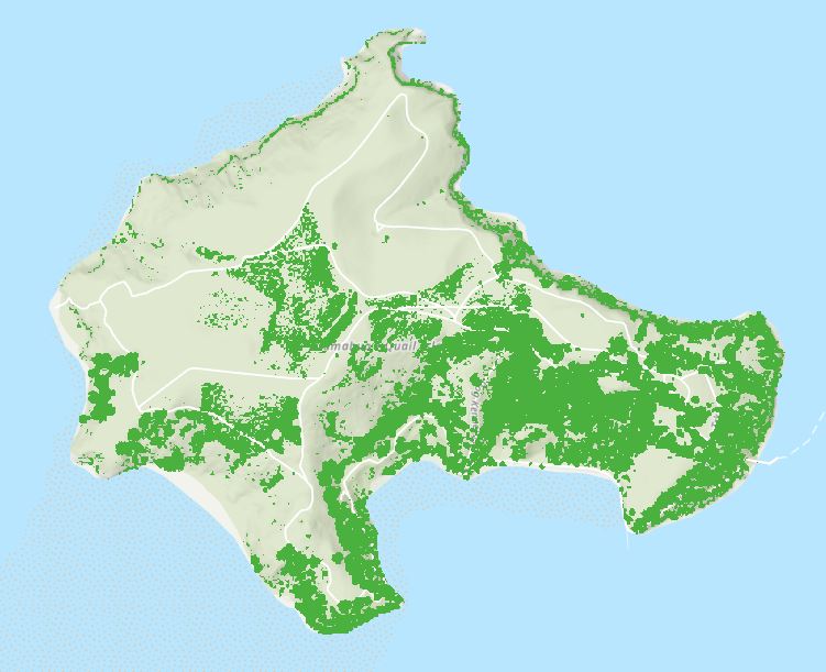
The darker green areas are vegetation greater than 3 m in height – for this analysis, it amounts to roughly 34% of the total island’s area. Not bad for (gulp) 26 years worth of hard mahi planting trees (Kia ora Quail Island Ecological Restoration Trust!). Given these data, we’ve actually got enough resolution to break these trees down into further height classes if we wanted to and, if we had data over time, we could track the rate at which trees are going in different areas. Nice.
Along the way in this analysis, I noticed a few interesting bits, which are actually the reason I’ve done this post at all – two things in particular.
When looking at the raw data points, I noticed that the range of elevations went from -1.2 m up to 539.63 m:
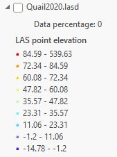
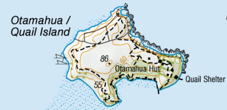
The max elevation was a bit of a surprise, as I know from the topo maps that it should be around 86 m (that’s ground level, mind you):
(The negative value is less of a concern as I know the data were collected around low tide, so -1.2 m is feasible.) But 539.63? What’s going on here? After a bit of visual examination, I did find a few out of kilter points:
See those two red balloon-like points floating high over the island? I think those are our culprits. There are often a few very noisy points in LiDAR data, but these seem a bit beyond the expected range. My guess? Birds are not an infeasible possibility. Yep, LiDAR could capture them in flight.
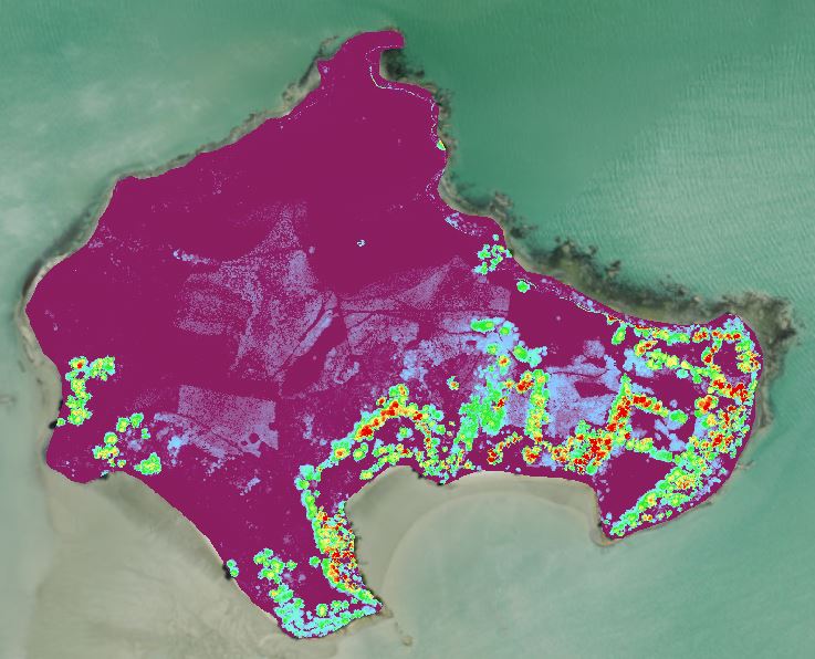
Another interesting tidbit – recall that to get our tree heights we’ve subtracted the DEM from the DSM – what’s left should be the tree height. When checking out my output from this step I noticed something odd – first the whole tree canopy layer:
No major surprises, except for a bit of an elevation hot spot along the northeastern coast:
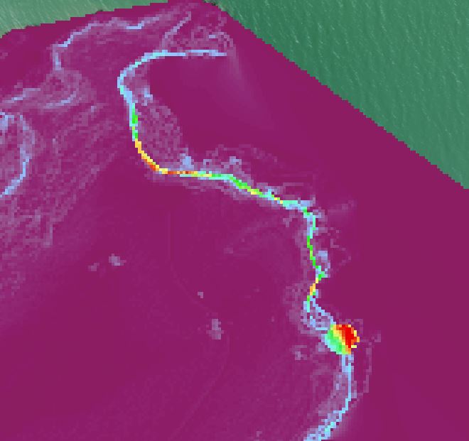
That oddly circular in shape at bottom right goes from around 20 m on one side to around 50 m on the other side – very odd. Closer inspection, reveals that there’s a tree there (image from Google Maps):
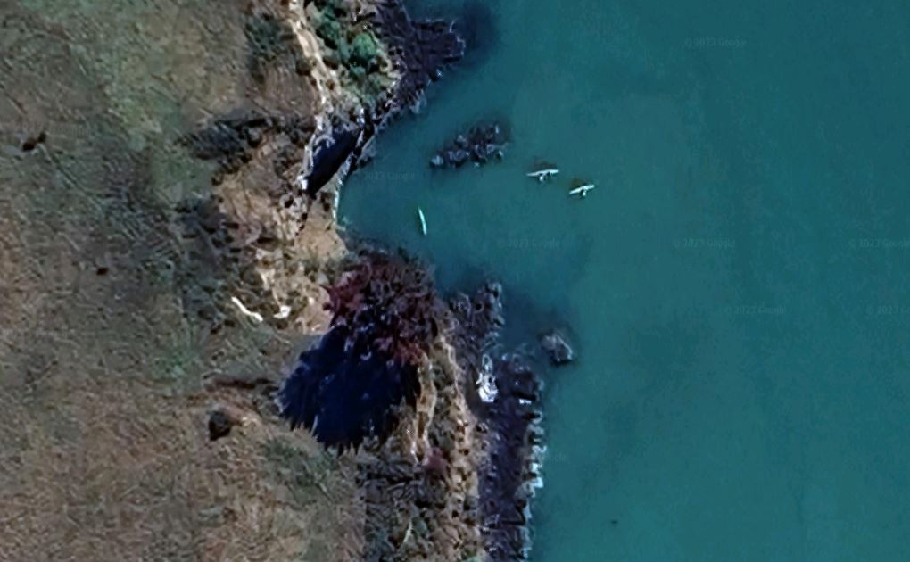
(Nice place to kayak!). At that location, the tree is a big one (a gum from memory) that overhangs the cliff, so for those branches that hang out over the cliff, the bare earth surface below is pretty much at sea level so it ends up seeming much taller there than it actually is after we subtract out the DEM. This is a fairly special case driven by the presence of cliffs and overhanging vegetation, but a good analyst will ideally pick up on these potential issues. One quick and easy way to deal to this was just to use a polygon layer of the island’s shoreline to clip out just the terrestrial areas:
You might think that this is just a bit of sweeping the problem under the carpet, but I think it’s a legitimate thing to do in this case.
So this has been another example of how LiDAR might be used for some very high resolution mapping, all made possible by the classification codes, and really just scratching the surface of what we can do with data like these. There was a lot of height in this post but hopefully not too much folly.
C