Zoning in on Landcover
We look at summarising vector polygon data within larger polygon zones using two different workflows.
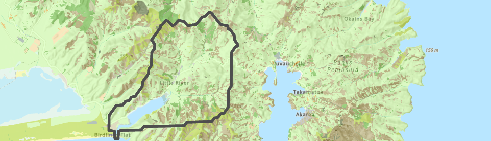
Polygons give us a handy way of creating zones, within which we might be interested in knowing what’s going on. Think of country boundaries, regions, school zones or even your own property boundary. Within those zones we often need to summarise some other phenomenon or physical characteristic. Suppose, for example, we’re interested in getting a breakdown of landcover within a river catchment. Sounds like it should be a pretty easy thing in GIS, yeah? Well, not necessarily. At least I haven’t found a straightforward way to do it yet so here I’ll outline two ways to do this. To give us some context, we’ll work with the catchment for Lake Forsyth/Wairewa on Banks Peninsula (which is composed of several different rivers and the lake):

I extracted this from the level 10 HydroBASINs layer on J:, just to give us something to work with. And here’s the Landcover Database layer:
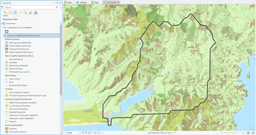
Clearly, there are a number of different landcovers within the catchment – my aim here is to quantify their areas and percentages within the boundaries of the catchment. Here’s a quick look at the LCDB attribute table:
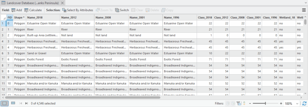
What I’m mostly interested in are the Name_ attributes. They tell me the name (or category) of each landcover with values for 2018, 2012, 2008, 2001 and 1996 (seems like we’re overdue of an update). Note too that there is a Class_ attribute. This has a numerical code for each landcover.
It’s a subtle but very important point that, even though this code is a number, it’s really just a category (the data mavens amongst us would call them nominal data). While we could add 22 and 21 (the codes for Estuarine Open Water and River respectively), the result doesn’t mean anything: what landcover is 43? It’s actually Tall Tussock Grassland, but adding the two doesn’t magically change the landcover – and Pro won’t stop you from doing this. Key takeaway here is that the Class_ attribute is a name masquerading as a number.
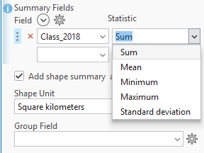
As a first cut it might be tempting to try the Summarize Within tool, which is designed to do just what I might want here: “Overlays a polygon layer with another layer to summarize the number of points, length of the lines, or area of the polygons within each polygon, and calculate attribute field statistics about the features within the polygons.” The only problem here is that this tool only works with numerical rather than categorical attributes, i.e. numbers rather than names. Let’s set the tool up so you can see what I mean:
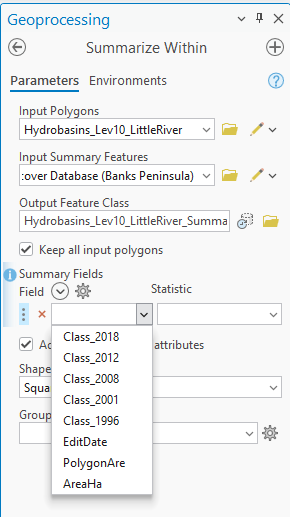
Under the Summary Fields, the tool only recognises the number fields. In the case of these data, I can make this work by setting the field to Class_2018 and the Statistic to Sum:
The output is a new polygon layer and the table looks something like this – I can only show a small part to make it readable:
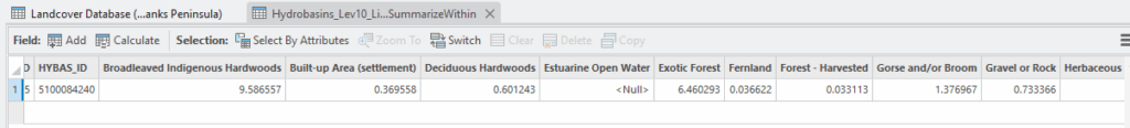
See how each of the class names is now a field? It’d be easy to assume that the values for each field are in square kilometers (especially as I’ve set the Shape Unit to these units) but they are actually percentages of the total catchment area. I only picked this up on a very careful reading of the help files. Note that since my input polygon layer has only one record, there’s only one output record – but there’s no problem with having multiple input polygons. For New Zealand, HydroBASINs at level 10 has 1,849 catchments which you could do all at once.
Summarize Within only works here because I’ve got my Class_ codes. But what if I didn’t have that? Let’s assume I’ve only got my Name_ attributes and still want to do the summarising? Here’s where a two-step approach comes in, namely by using Tabulate Intersection followed by Pivot Table. Let me explain.
Tabulate Intersection does just what it sounds like – it “Computes the intersection between two feature classes and cross tabulates the area, length, or count of the intersecting features.”:
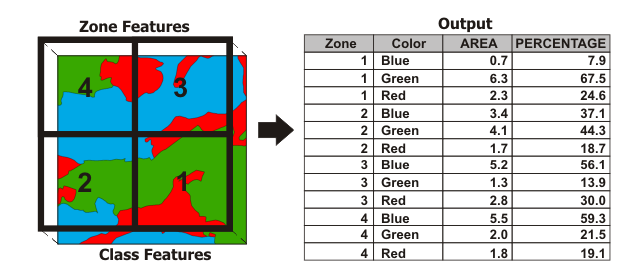
The Zone features are the polygons we want to summarise within while the Class features are what we want to summarise. In the output (which is a table) each Zone can have multiple rows – one for each class within it. Plus, we get Area and Percentage in one fell swoop. Let’s try it on our Little River Catchment:
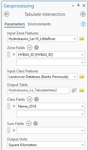
I’ve set the Zone Field to HYBAS_ID. This is a unique identifier for each catchment in this layer. This will become more important when we use Pivot Table (I could have used OBJECTID as well). Here’s the output:

As we may have expected, we’ve got a record for each Name_2018 value with AREA and PERCENTAGE fields and all the HYBAS_IDs are the same. This has tallied things up for us nicely but as a next step, we’ll attach these back to our catchment polygon using Pivot Table.
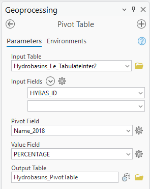
This tool works just like it does in Excel – we can reorganise the table and “flatten” this many-to-one relationship. This image from the help file may help:
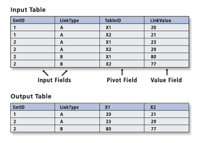
I’ll be honest, whenever I use this tool I have to think hard about which field is which and often have to run it a few times to get it right. What I’m wanting to do is to convert this table of 20 rows to just one, with a column for each landcover’s AREA and PERCENTAGE. The only drawback here is that I can only do AREA or PERCENTAGE, not both. Here I’ve set it to do the PERCENTAGE:
The output is, once again, a table:
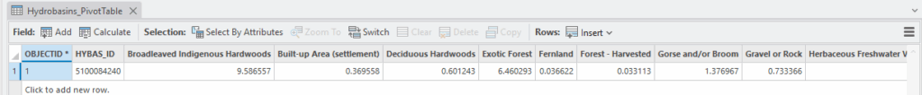
If I need this as part of my polygon layer, I can next use a table join to link this back using HYBAS_ID, giving me a breakdown of the percentage area for each landcover. Again, if I had multiple polygons in my input layer, I’d also have a breakdown for each one.
We’ve looked at two ways of summarising one layer’s polygons within a different set of polygons: Summarize Within and Tabulate Intersection/Pivot Table. Each can be made to work and which one you choose will depend on what attributes you’ve got to work with. As another example, I was recently wanting to do something similar with zoning data within a town boundary. The input data had categories of planning areas but no numerical code to go with it. My only option was Tabulate Area/Pivot Table so, once again, Analyst, know thy data.
We’ve got a few other things to cover while we’re talking about summarising data within polygons, especially when it comes to raster data (spoiler alert: zonal statistics). But that’s a job for another day.
C
