Challenging Times – Challenging Patches
We dissect how to approach a challenging spatial problem by relying on some basic levels of analysis.
We often get a lot of challenging problems of a spatial nature here in the GIS world. A common thread of these is that they often sound easy at the start but get much more complicated when you try and come up with a solution. In this post I go over one posed to me recently which ended up being a particularly challenging but satisfying one to solve. Warning to you, oh gentle reader – this is a long post with some code snippets but I do promise some pretty pictures.
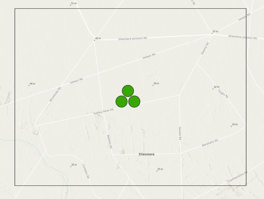
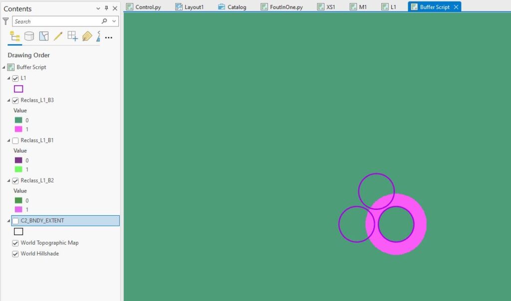
Over the past few months I’ve been working with a colleague to develop a script for their analysis. The research is around ecosystem services and how different configurations of bush can enhance their effect. So this means a lot of testing of different configurations and comparing the outputs. Richard (said colleague) is focusing on four ecosystem services and has its own set of equations to model their effect based on different configurations of bush. Here’s an example of one of the simpler configurations – three polygons within an area, called L1 – purely hypothetical – and the study area boundary:
With at least 16 different configurations consisting of three, nine, or 900 patches of bush and four ecosystem services, this is a task that cries out for automation, using either ModelBuilder or a custom Python script. We quickly determined that this was too much for ModelBuilder and got onto the script.
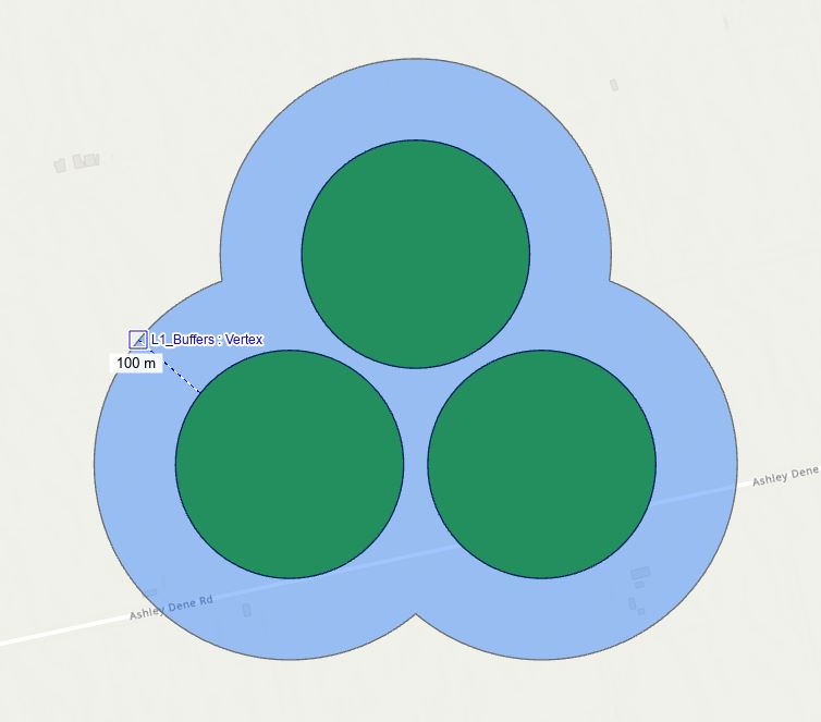
Before we get to any that fun scripting stuff, maybe an example would help. There are four ecosystem service effects that Richard is looking at: cooling, habitat for both Bellbirds and Fantails, and nitrogen. Each has its own set of equations that model the effect, driven mainly by distance away from the patches. If we look at Fantails, an assumption is that the effect of a patch of bush extends out 100 m from the edge of the patch, so we’re really interested in what happens with that 100 m zone – like this:
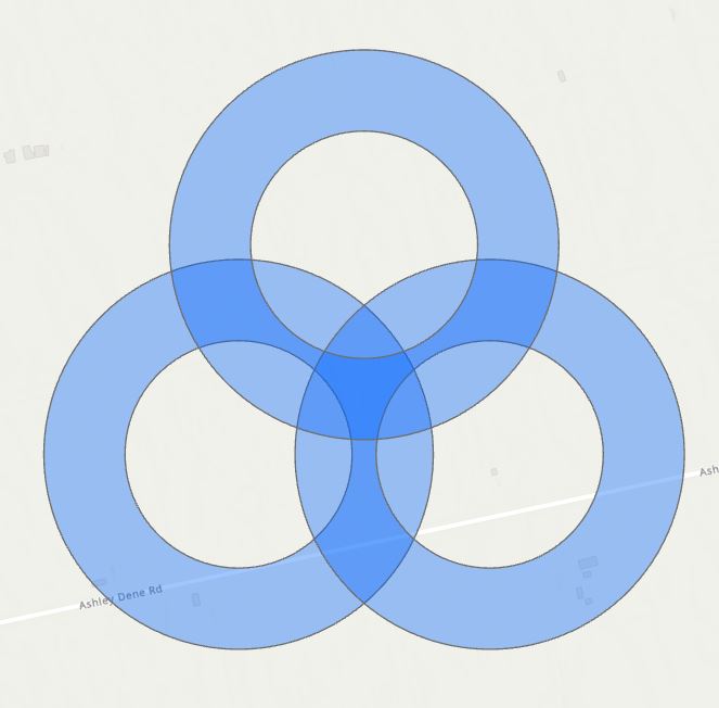
This has been very much a work-in-progress with me writing a script, then Richard testing it and gradually working out all the things that don’t work correctly. Most recently this meant looking at areas where the ecosystem service effect from each patch overlaps with other patches and doing additional calculations within that overlap – an attempt to reflect how these overlaps can enhance the effect. The focus here is more on the edge than on the patch itself so the outputs need to exclude the patches themselves
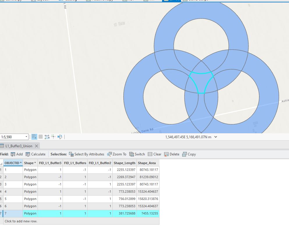
Now we’re looking at something different from above – the focus is where the individual patch buffers overlap, so we’ve got to look at each individually and together:
(John Bonham anyone?) More specifically, we need to focus on the areas where these three overlap while also excluding the areas inside each buffer, so the dark blue areas:
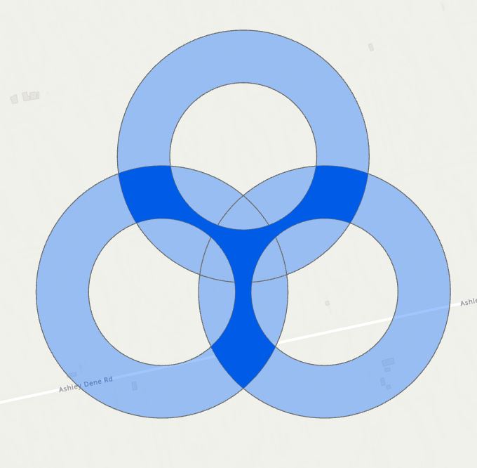
Within those dark blue areas, the additional computing needs to be done, but only there; everything else needs to keep their original values.
It’s probably worth saying at this point how I got the image above – it wasn’t trivial. In brief:
- Buffered each feature individually by manually selecting each in turn (and setting Side Type to “Exclude the input polygon from the buffer”
- Unioned the three outputs
- Manually selected the features in the overlap and exported those as a new layer
- Manually selected the pieces that ended up inside a patch boundary and deleted them
- Could have gone one more step and dissolved all the internal boundaries but just used symbology to make it look like one polygon
Note that a lot of what was done above involved me deciding which polygons were important. Doing this manually with L1 was not too challenging but I did make a few mistakes along the way. But doing this manually with 900 features (and doing it correctly) is just plain madness.
And that was the real challenge posed to me. How can I make this work in a script in an automated way regardless of the number of patches and their configuration? I can’t always be there to make the decisions so I will have to come up with an objective way of doing this that only makes use of what’s in the data. This thing has to function on its own in the real world.
When starting a new script my approach is often to figure out how I would do it manually and then decide how to make that happen in the script. Here the first big choice was vector versus raster, and my initial thought was to use vector with buffering and spatial joins. What I did above to create these images was pretty much what I tried first. While it could be done manually, it was apparent that it would be very problematic to do this programmatically, mainly because it relied on someone being able to make decisions, on the fly, about what’s important. Looking at the attributes, I didn’t see anything that I could easily use in a bomb-proof way to end up with the right areas. Here’s the attribute table from the Union:
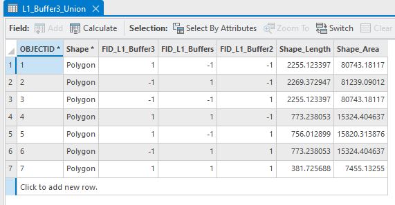
You can see a field for each of the input layers with a 1 if it’s from that layer and a -1 if it’s not. Can I somehow use Select by Attribute to find all the right overlap polygons?
I can say for sure that the record with three 1s is where all three overlap, but there are plenty of other combinations that should be included and the ones that should not. The thought of coding this logic makes my head hurt. And this is just three patches – what happens when I get to 900? I think with enough effort this could work, but getting the logic right feels like a nightmare, so let’s try raster, eh?
The good students in ERST202 and 606 might be quick to think of using Euclidean Distance and then Reclassify (heaven knows we’ve been doing a lot of that lately (Ed. Poor souls…). And that’s a viable way to do it, but at this point I’ve already got some buffers so I’ll just convert each of those to raster using Polygon to Raster.
A funny thing with this tool – I need to explicitly set the extent and also take care with the output, as I’ll get some grid cells with a non-zero value within the area of my buffer polygons, but everywhere else will be NoData. If I use these rasters in some calculations, those NoData cells will stay NoData all the way through, essentially blanking that cell out for all future calculations, so I’ve got an extra step of setting the non-zero cells to 1 and the NoData cells to 0. I end up with three raster layers of 0s and 1s, one for each buffer:
(I can only show you one raster layer at a time here but hope you, ahem, get the picture.)
So with 0s and 1s I could think about Boolean Operations (AND, OR, XOR) and I next tried each in turn.
With an AND I should get 1s only where it’s a 1 in all three inputs, so:
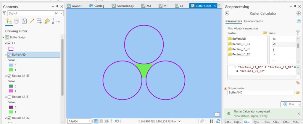
(This would be the same result from a vector Intersect, by the way.) This is part of the overlap, but only where all three do, so only a partial answer. Let’s try and OR – with this, I should get a 1 wherever any of my input layers has a 1, so
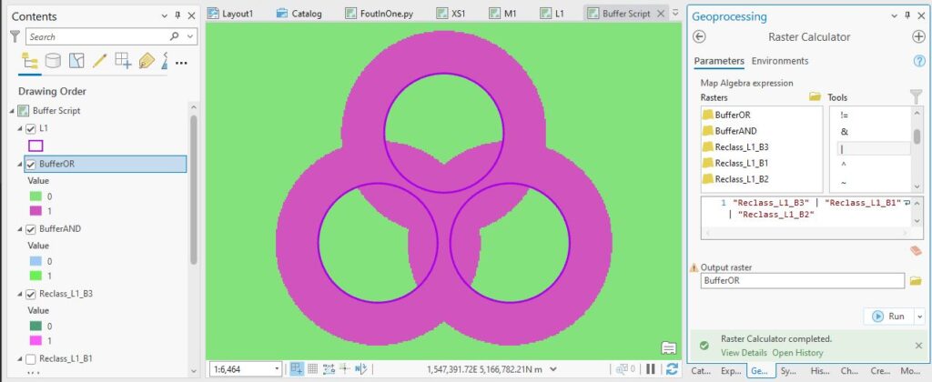
Bit too much here – I’m even further away from something I can work with. One more to try, XOR. With this Boolean I get a 1 where there’s no overlap and 0s where there is, so it’s sort of like a vector Erase (and your first pretty picture):
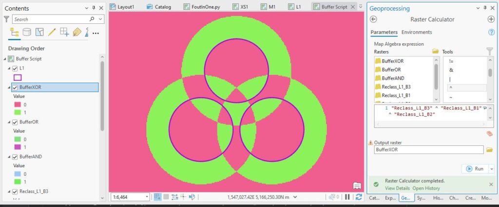
I’m no closer to a solution. Even a fancy reclass won’t get me out of this mess, so I think I’m done with Booleans. Moving up the food chain of operations, let’s try some Map Algebra – I’ll just add the three rasters together:
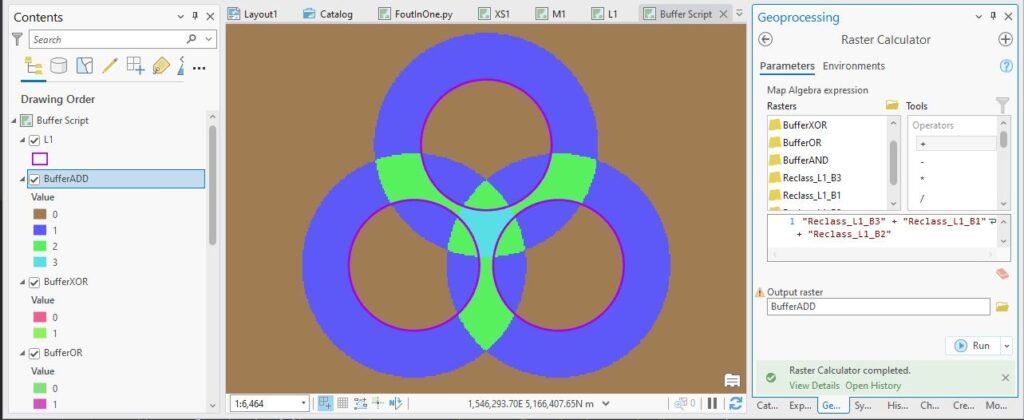
Oh my, for the first time I feel like I’m getting somewhere. Looking at the output values, the 2s and 3s are the areas I’m interested in. 0s are outside the buffers and 1s are where there’s just one buffer, so with a quick reclass, I’ll get a layer that just about gets me where I want to be:
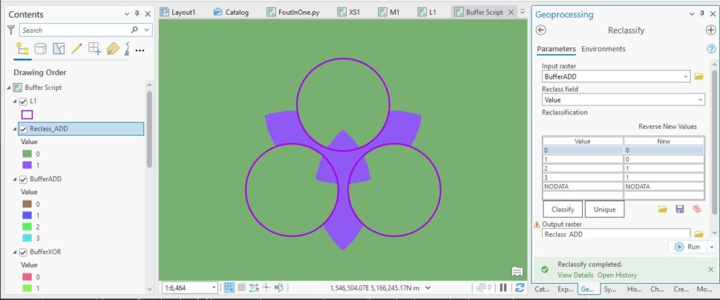
What ho – just about there. But you can see I’ve still got some bits that extend into the three patches which I need to remove.
As it turns out, as part of the script, I was already creating a raster layer where the area within each patch had a value of 0 and everywhere outside was a 1 (called SPUMask.tif), so with one little multiplication I can do away with those annoying bits:
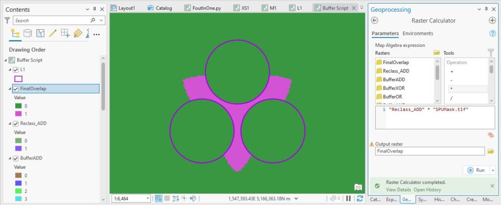
Eh voila! I’ve got a layer that I can use to tell the script where to do its extra enhancement calculations. And I’ve gotten there from the bottom up, starting with simple vector and raster tools to settle on something that I can now work into code.
The code-averse amongst you might want to look away now, as I’m going to go into the gory details on how that ended up working in the script.
Thinking about the Python script
So I’ll summarise the key steps here with thoughts on what tools I can use in the script:
- Create a vector buffer around each patch – for this I need a loop that cycles through each record (patch). Running the Buffer tool for each selected record gets me one for each patch.
- Convert each buffer to a raster layer – Polygon To Raster works provided I set the extent and the output cellsize
- Reclassify so that the NoData cells get a 0 and everything else gets a 1
Those three steps happen in the loop, once for each patch. With the L1 configuration we’ve been looking at I get nine outputs: three individual vector buffer layers, three raster versions of the buffers, and three reclassified raster layers with 0s and 1s.
- Outside the loop, I can then add them all up. With L1 I get values ranging from 0 – 3, as we saw above. (Gotta be careful here – with other configurations I may get larger maximum values than 3.)
- Knowing that 0s and 1s should be 0 and anything greater than 1 up to the max value should be a 1, I can then reclassify that layer into 0s and 1s. The 1s are my areas of overlap (regardless of the number of overlaps) and 0s are where there is either no overlap or at least one buffer area.
Once I’ve got this layer, I can then use it as a bit of mask and tell the script to do some extra calculations within the area of 1s and leave the rest of them alone. Pretty much job done, methinks.
Next steps are to incorporate this into the main script, tie up the numerous loose ends this creates and test it out.
The Python script
Code-averse folks that are still with us may now want to leave the room, unless you’re wanting something that may help you get to sleep. Here’s how the script looks (only showing the code for Fantails for clarify here but each of the ecosystems gets a similar treatment – line numbers won’t be consecutive).
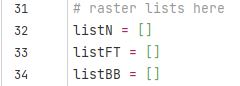
I first need a list for each ecosystem service to store the output grids temporarily so I can later add them all up when all the patches have been processed.
Each time the loop runs its last job is to add the output raster to the correct list.
Next we set up the loop to go through each record in the patch layer (inputFC), one by one. A SearchCursor does the heavy lifting of iterating through each record in the inputFC and also reads in various attribute fields, e.g. OBJECTID. fid = row[0] grabs the OBJECTID which is used later to create output names. The script moves to the next record at the bottom of the loop, continuing until it reaches the last record. arcpy.env.workspace = ws tells the script to save outputs to a specific folder:

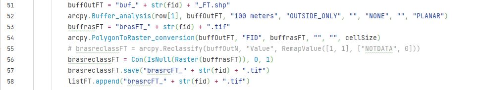
The next block does the buffering, conversion to raster and reclassifying, saves the various outputs and adds the final raster to the list for Fantails (well, the list actually does that) for each record:
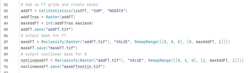
Once all the records have been processed, we exit the loop and add up all the layers in listFC (using CellStatistics), find the maximum value in that layer (addFTras.maximum – I don’t know in advance how many overlaps I might get – this solves that problem), then reclassifies it using the logic we talked about above (I haven’t ended up using the outputs from lines 87 and 88 – they’re for another purpose. Lines 90 and 91 finalise the overlap mask for our purposes.)
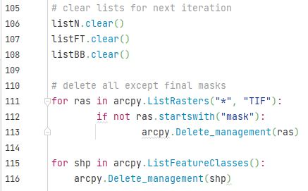
Now, with the result we need, the script clears the lists and and deletes what we don’t need anymore (the vector buffer layers and all the intermediate raster layers) just to keep things tidy and save on space.
Job done! I won’t inflict the full script on you (Ed. Again, thanks); it’s quite a beast and easily the most complex I think I’ve done yet; lots of moving parts, including my sanity.
In many ways, it was very satisfying to get this working (Ed. counselling is available…). What sounded like it should have been simple at the outset ended up being a lot more complicated and challenging. On top of that, solving it meant going right back to basic kinds of analysis and a bit of playing around to find what worked best. Some testing gave me confidence that it was actually working as advertised and so far so good as Richard works through his configurations.
Now if I could just regain my usual Zen sense of calm (ha!)…
C