Carnival of Coordinates
We struggle with a point dataset’s coordinate system and delve into UTM.
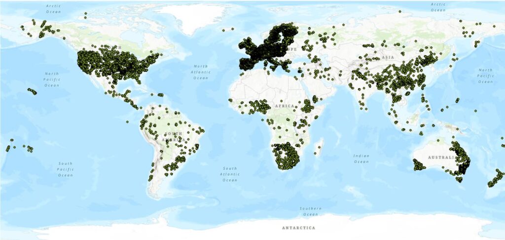
Ah, if only every day could be a carnival at GIS Central…sigh. Rather than a samba to start the day, here’s a fairly common occurrence: a colleague sends me some data in a CSV file and asks me to map them. As usual, sounds easy, but… We’ve been continuing with more of the global data modelling, this time looking at world-wide estimates of available phosphorus in soils and, hence, which areas could benefit from reduced applications. Thus far, I’ve got a dataset of 44,380 points we’re using to extract variables related to climate, soils, cropping, runoff, and a host of others which will then be used to develop a predictive model – here are the points:
These were mapped from a CSV file that looks like this:
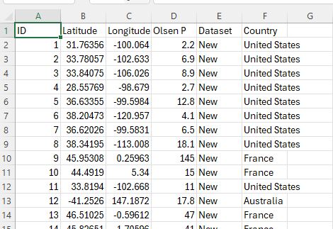
Nicely formatted data with Latitudes and Longitudes in WGS84. Life is good, almost a carnival.
But arriving in my inbox one sunny morning was a new CSV file with some new data from Brazil (Ed. oh my, how exotic.) They looked like this:

At first glance, things look okay – most importantly I’ve got a column for Latitude and one for Longitude. There are 364 points in all so not too onerous. On closer inspection, though, a question arises. What the heck are those coordinates in? That ain’t latitude/longitude. In order to map these I’ll need to know, so we’re in some familiar territory.
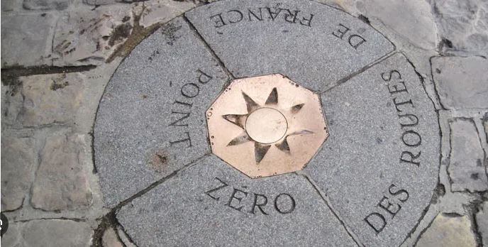
From the look of these numbers, I’d guess that they are from a projected coordinate system so it could be one that’s been designed for use within Brazil, like what we use here, New Zealand Transverse Mercator (NZTM). Or they could be in Universal Transverse Mercator (UTM). After a bit of digging on the internet, I couldn’t find anything like NZTM for Brazil so headed down the UTM road. UTM, similar to our own NZTM is coordinate system that enables any feature on the surface of the earth to be located unambiguously with two coordinates: one in the x-direction (an “Easting”) and one in the y-direction (a “Northing”). Any coordinate system needs an origin, the point with coordinates (0,0), and the point from which all the measurements are made, sort of like Point Zero in Paris.
And here it gets complicated for UTM. We’re back to the classic problem of taking a very large, spheroidical object (namely, the Earth) and forcing it to be all nice and flat. You simple can’t do that without distorting things in one way or another. To minimise this distortion, UTM breaks up the planet into 60 zones, or fuses, each with its own origin and spanning roughly 6 degrees of longitude. On the global scale it looks something like this:
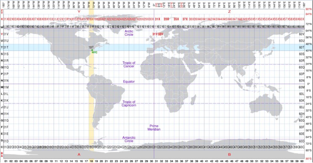
Zones are numbered west to east starting a 180 degrees, just to the east of us. As we’ll see later, each zone is further divided into North and South of the equater, each with their own set of coordinates. To make matters worse, each zone is also divided up in latitude bands, designated with letters starting at C in the south and going up to X (but avoiding O and I to reduce confusion with the numbers 0 and 1), so any location will be within a particular zone. The South Island, for instance, fits almost entirely within zone 59G. (We can also say that it’s in the 59S zone, S for South) On the figure above, New York City is in zone 18T (and also in 18N).
Thinking about origins, each zone’s origin is set where its central north-south line (meridian) intersects with the equator. To avoid any negative numbers, the origin is assigned a set of false values such that every x- and y-coordinate in the zone has positive values. Importantly, each zone has it’s own projection. What this means is that any given set of coordinates could be within any one of the 120 north or south zones: one really needs to know which zone we’re talking about if we want to map them.
If we go back to our CSV we can see that, in addition to the coordinates, each record also has a “fuso” value. Now I don’t claim to speak Portuguese, but I’d be pretty sure that this refers to our UTM fuses, and these match zones in Brazil, so hidey ho! My points span the 22J, 22K, 23K and 24K latitude bands, so let’s see where those are on a UTM map (I added this from Add Data > Browse > ArcGIS Online > World_UTM_Grid):
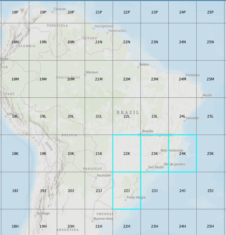
We’re zeroing in – these give me a good sense of where my points should be if I get their coordinate systems assigned properly. We’ll come back to this map in a bit.
So, where to with these data? I’ll want to get some points on the map, and given that I’m starting with a CSV, the next steps are to add the table to a map and use Create Points from Table > XY Table to Point. We said earlier that each zone has its own projection, which I’ll need to set with this tool, meaning I have to treat each “fuso” separately. This meant starting a new table that just had zone 22J points, a separate one for 22K, one for zone 23K and one for zone 24K. Once done and added to the map, I can open the tool and map each set of points individually:
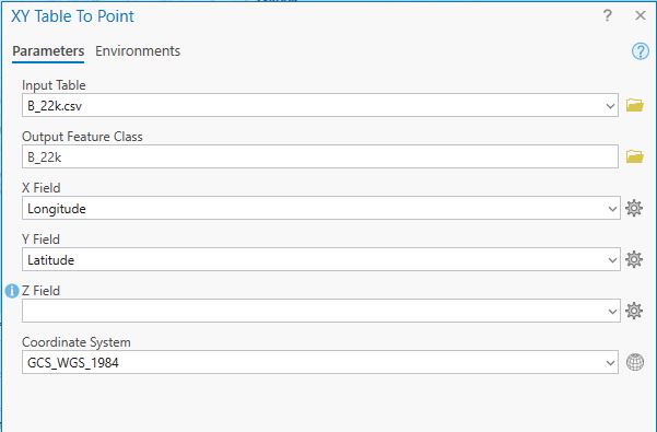
(The “B_” is for Brazil.) By default, Pro sets WGS84 as the coordinate system. To change this, click the Globe icon:
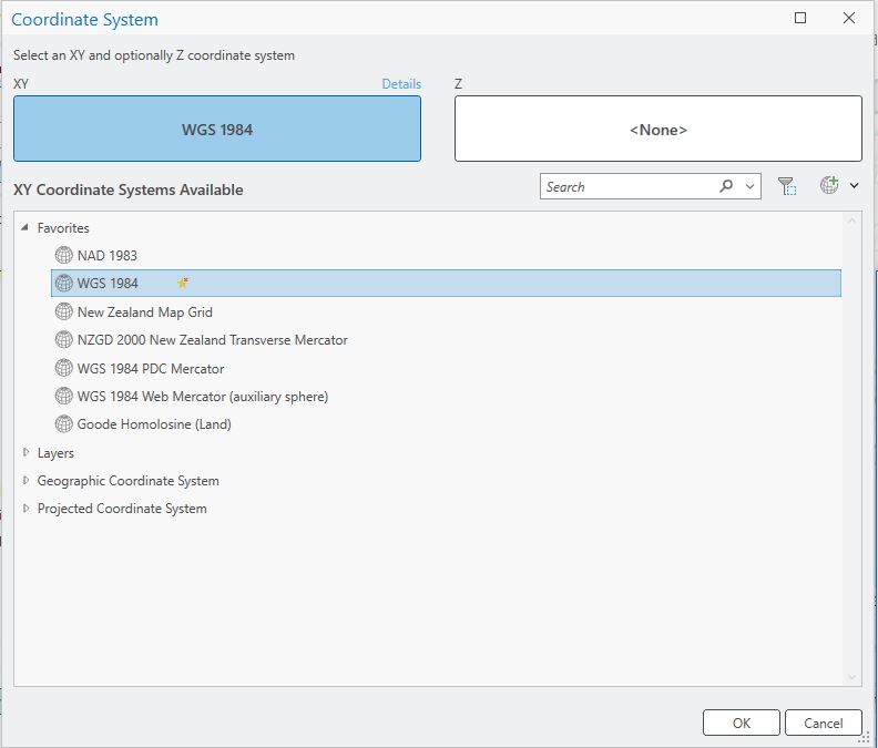
To find UTM, go under Projected Coordinate Systems > UTM > South America. This lists about 30 different coordinate systems – here’s a smattering:
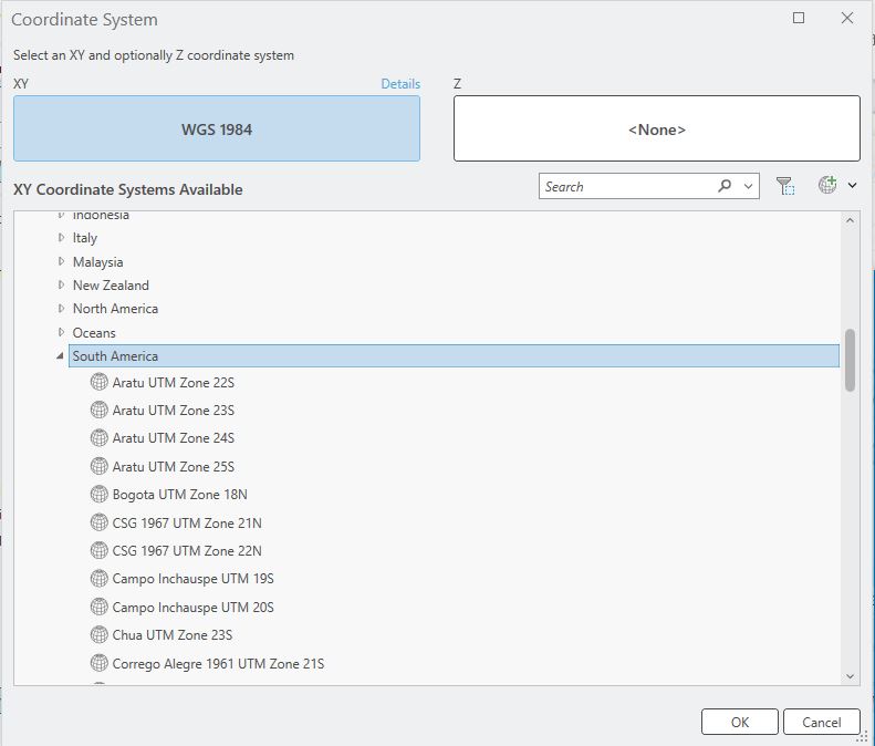
There’s a dizzying array of systems to choose from, so after a bit more digging, I concluded that the best system to use for Brazil was called SIRGAS 2000 (Geographic Reference System for South America) – with a separate UTM projection for each zone.
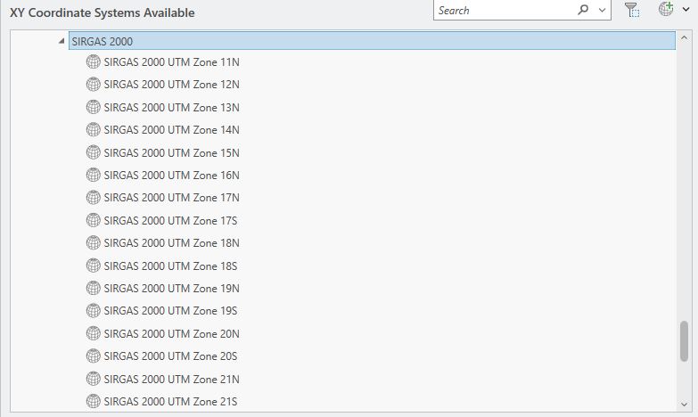
The eagle eyed amongst you may have picked up something interesting here… I know I’ve got zones in the J and K latitude bands but the only projections available here end in N and S. What more can a poor boy do? (Why are there norths and souths available for South America? Because the equator does pass through the continent – that’s where Ecuador got its name from.) It’s not entirely clear to me why the latitude bands are not treated separately here but we must conclude that when it comes to UTM projections, we only have North and South to choose from, something Carlos Grohmann takes issue with, and I think he should know. Okay – so I’m a few steps away from points on the map. For each set of points grouped by fuse, I can set the correct projection and add the points – you can see that they nicely fit in the correct fuso:
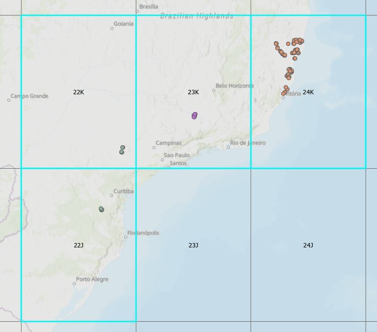
(I did look for some independent confirmation that these were correct but the only thing I had to go by was a figure from a paper (figure 1) that couldn’t confirm things for me, so we’re going on a bit of faith. But I did do a bit of inspection – found some points that fit very nicely over a wooded area}
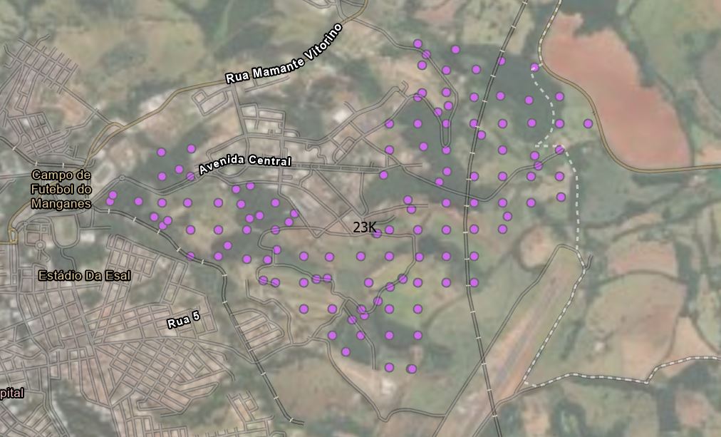
But we’re not out of the woods yet. Before I can merge these points in with the other 44,380 I need to have their coordinates in WGS84. No problem – Pro can do the transformation for me in the attribute table. Next steps:
- Add two new fields (Latitude and Longitude) as floats to the each layer’s table
- Right-click on one of the attribute names and chose Calculate Geometry
- Set the output coordinate system to WGS84 and point them at the the correct fields
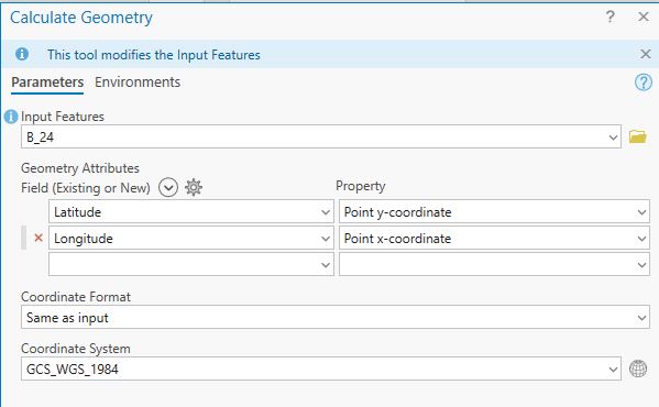
After clicking Run, the coordinates are added to the table:

These tables were then exported as CSVs and combined into one file (with a good bit of quality assurance) and then added to the original CSV for remapping. Job done. I’d show you the output but it really doesn’t look a whole lot different to what I showed at the beginning of this post.
So, once again, what sounded like a simple thing to do ended up down a bit of a UTM rabbit hole but all good in the end. I learned things about UTM I didn’t know before (and Brazil for that matter!). And it does highlight the importance of coordinate systems when handling new data. (I will say that my first attempt at this had several points happily floating in the South Atlantic but that was definitely user error.)
The worst part about this whole effort was that the closest I came to Carnival in Rio was on a map. (Ed. oh, pooooor you…) Perhaps I need to go and do some ground truthing. Yeah, that sounds like a good idea.
C
