Overflowing with River Data
We review several digital river networks and how they can be used.
Spatial data for rivers are one of those fundamental data layers needed for many different kinds of analysis, along with elevation and landcover. Over the years there have been a few different datasets available so we’ll do a quick survey and see how they’ve changed over that time.
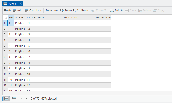
When I first started playing this GIS game, the layer of choice was from the LINZ Topographic Database – a layer called river_cl.shp. (You can find a copy on J:\Data\Toposhapefiles.) (Ed. That is soooo last century…) This layer showed the locations of rivers and streams based on the 1:50,000 scale topomaps from LINZ. They are just digitised versions of what we can see on the maps:

Attribute-wise, there’s not much to it:
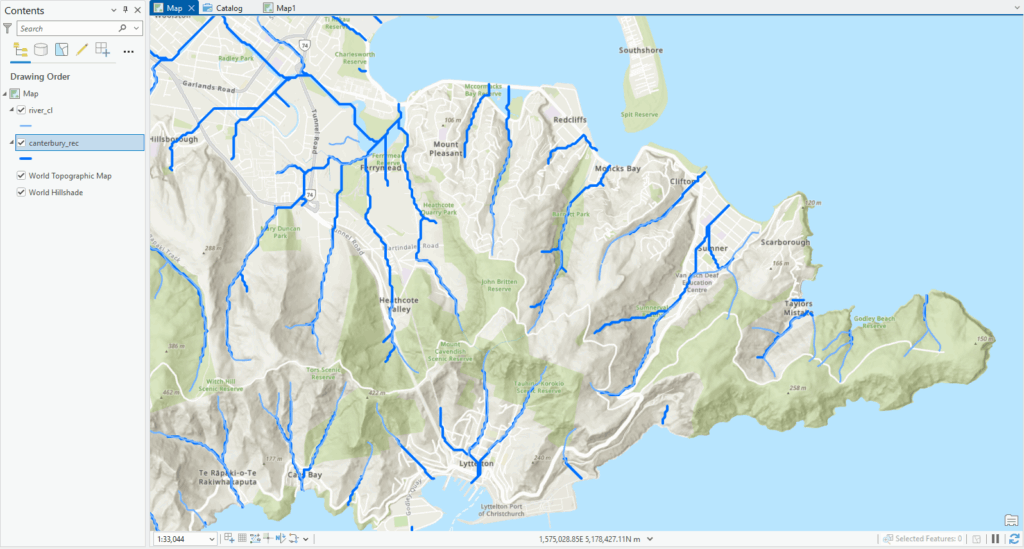
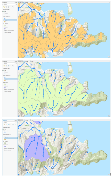
This was fine if all you needed were lines on the map but didn’t offer much by way of analysis. In 2004, our friends at NIWA developed the River Environment Classification – a laudy attempt to update the river network but also group river reaches into categories related to six key variables: climate, source of flow, geology land cover, network position, and valley landform (J:\Data\River_Environment_Classification). Now we could not only show river locations, but use these categories to group rivers by similar characteristics in a hierarchy of variables. Here’s the REC shown with river_cl – the darker features are REC so, in this area, streams extend to the sea and additional reaches are visible (these data are in the Classifications folder broken up by region):
For attributes, the table is brimming with info:
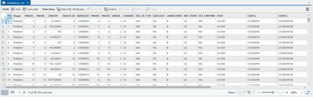
NZREACH is an important attribute here. It’s a unique identifier for each section of a river. To the right you can see values for each of the key variables (decoded in the user’s guide PDF) and even further right you can see different groupings that get to finer detail as they build.
And along with the lines, we also got polygons for catchments at different scales (in the Catchments\All_river_orders folder), more specifically at different stream orders.
These were useful but one often had to do a bit of trial and error finding the right size catchment for specific purposes. (Here’s roughly how those catchments were created.)
Fast forward a few years and along came REC2 (J:\Data\River_Environment_Classification_2) with a more extensive river network though the loss of the categories from the original REC1 layer (look in the nzRec2_v5 geodatabase. The Hydro feature dataset has the riverlines). To make matters challenging, NZREACH was replaced by nzsegment and they are different, so the same river (on the map) could have two different IDs, making them difficult to link up. This led to all sorts of fun and games which weren’t necessarily fun. (Ed. Stop gritting your teeth, let it go.)
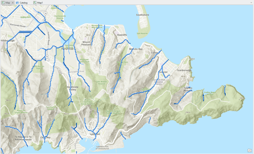
(REC2 is darker here so a few extensions to REC1). Also with this version, we got a new set of catchments (in the rec2_watersheds feature dataset), one for each river reach in this versio. Both have the same unique ID (now called nzsegment) so we can link them together using this (it’s a messy image, I know):
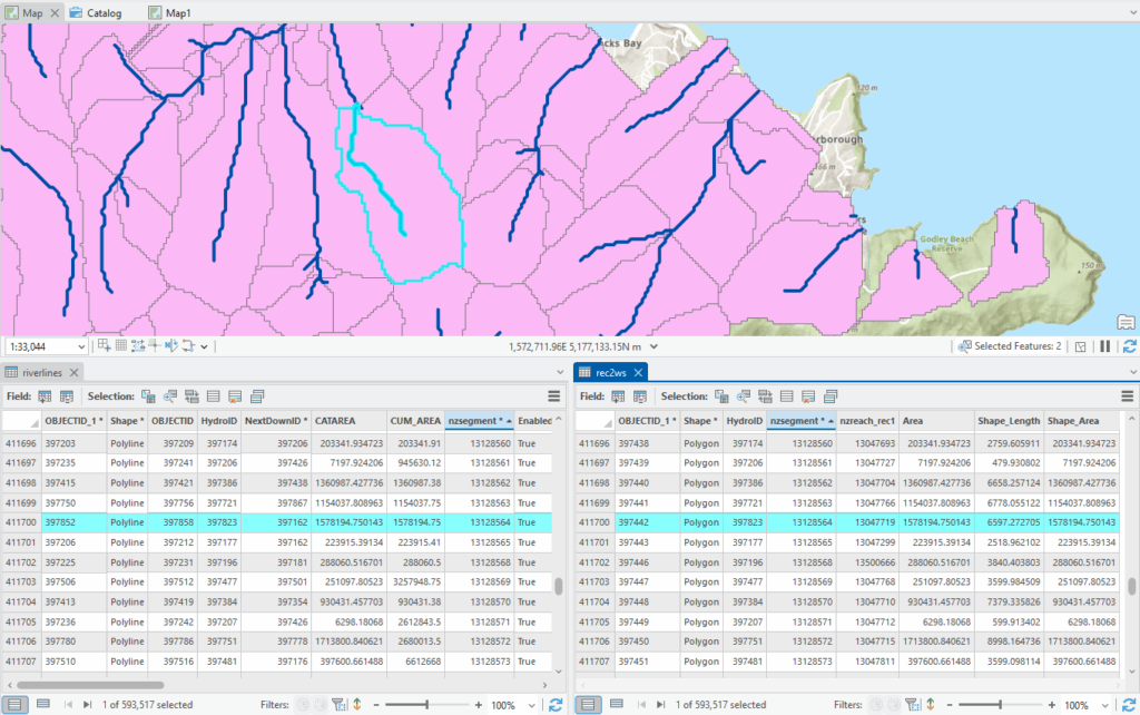
Having a catchment for each reach means that we can build up our own catchments as needed (whether that’s a plus or not, I’m still deciding.) To do this we’d have to first select the river reaches of interest, then do a Select by Location, then export those catchments and finally use Dissolve to get one overall catchment. Bit of a pain, that.
The riverlines in REC2 don’t have the same attributes as REC1, but they are still available as standalone tables within the nzRec2_v5 geodatabase:
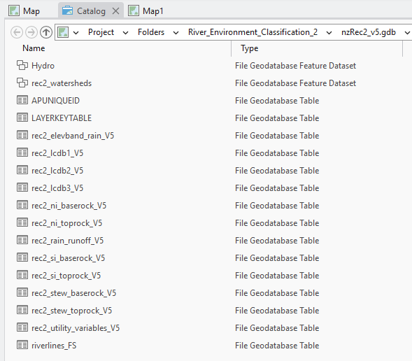
REC2 is jam packed with useful information from those standalone tables but does require the user to have their wits about them. The tables are mix of island-specific data (e.g. rec2_ni_baserock_V5 has geology just for the North Island. “stew” is for Stewart Island.) It’s hard to make sense of what the attributes mean unless one looks at the rec2_attribute_definitions.xlsx file in the REC2 folder. As an example, for ni_baserock below, the Description links to the abbreviations in the table:
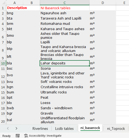
Looking at the layer’s table, we can see the different rock types across the top and the link to each river reach:
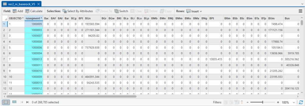
Non-zero values are the area in m2 for each rock type for that reach’s catchment. We can link these records to the spatial riverlines using the nzsegment attribute and a table join.
The rec2_utility_variables_V5 table has some useful climate variable for each reach and catchment. The Utilities tab in the Excel spreadsheet decodes the attributes:
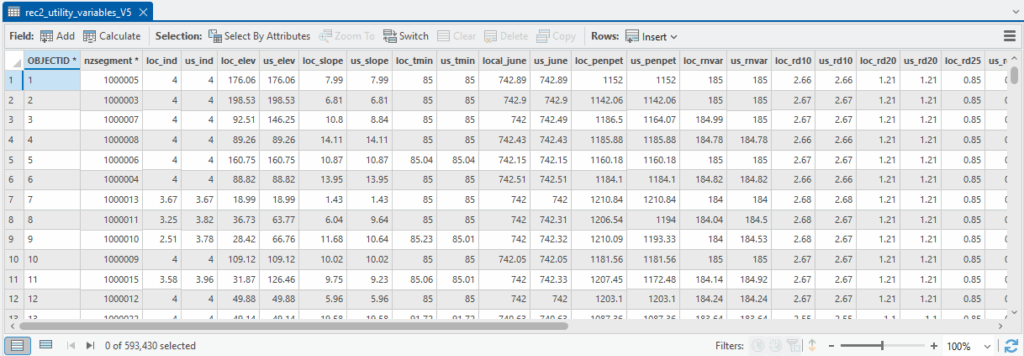
(“loc” stands for local, or that particular reach, while “us” relates to that reaches upstream area.)
One other nifty thing about REC2 is that there’s a trace network layer in the Hydro feature dataset, meaning you can use this to trace up- or downstream within the network – we looked at this once before using network datasets and trace networks work similarly.
Most recently, I came across NIWA’s latest version, the Digital Network (version 3) (DN3). This one provides even further refinement of the river network and a new set of catchments (J:\Data\DigitalRiverNetwork)
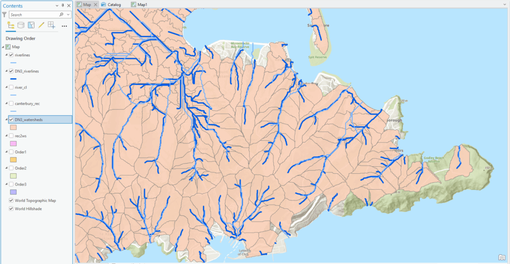
Lots of additional reaches and a significant increase in the number of catchments. Whichever version you or REC/DN you look at, one thing you’ll be able to find in all of them is a stream order attribute. Cartographically, it’s nice to use these to help indicate the relative size of a stream using Graduated Symbols as shown below:
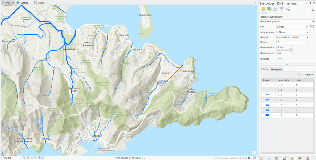
Visually, I find this layer the most appealing in that it’s smoother and more extensive – probably the result of using higher resolution data. At this point, the extensive variables from REC1 and 2 don’t yet appear to be available, so I’m probably sticking with REC2 for analysis and DN3 for visualisation.
The data for DN3 are downloadable from the relatively recently formed National Environmental Data Centre – you should have a look at what’s available there. We’ve got a copy of DN3 on the J: drive but you’re also welcome to add it directly to a map as a web service. Here’s how
- Go the NIWA Open Data portal and search on DN3 (another nice data portal in the mix)
- Select the region of interest, e.g. Canterbury
- Click on View Data Source
- Copy the URL from the address bar (here’s one I prepared earlier: https://services3.arcgis.com/fp1tibNcN9mbExhG/arcgis/rest/services/NIWA_DN3_canterbury/FeatureServer)
- In Pro, click the dropdown menu under the Add Data button and choose From Path…
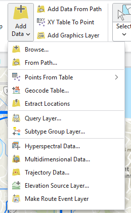
- Paste the URL in to the Path window and then click Add
This adds both the riverlines and the catchments layer. You can always export them to your project geodatabase if you need a local copy or copy it from J:.
Well that’s enough of that! More about rivers than most people really want to know.
C