That Cat(fish) Scratched Back
We look at extending our marine ecoregion polygons to get more observations categorised – not as straightforward as it might sound.
In a previous post we looked at extracting data on marine ecoregions to a set of observations points. For the most part it worked pretty well, but out of our 2million+ points, around 200,000 had no data (~10%). Visual inspection showed that many of these points were around large, inland water bodies, like the North American Great Lakes, while others were close to shorelines but some distance inland. On advice from marine scientist Chad, we thought we might extend the ecoregions 20 nautical miles (nm) inshore to try and reduce this number as much as we could. Some of these observations could be in inland freshwater lakes or in estuarine areas of rivers, or quite possibly just in the wrong place.
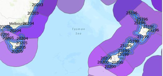
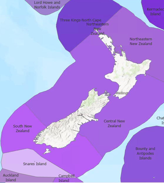
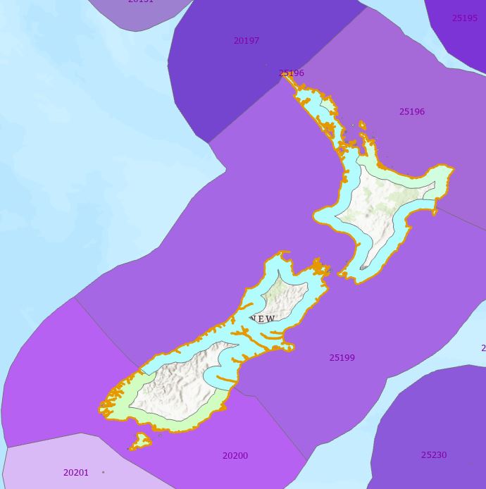
And therein lies a classic GIS phenomenon: it sounds like this should be an easy thing to do but is actually quite challenging. Surely I could just buffer the ecoregions? Well let’s first look at that to get this post rolling. First, here’s the Marine Ecoregions of the World (MEOW) for our little part of the globe labelled with the Ecoregion names:
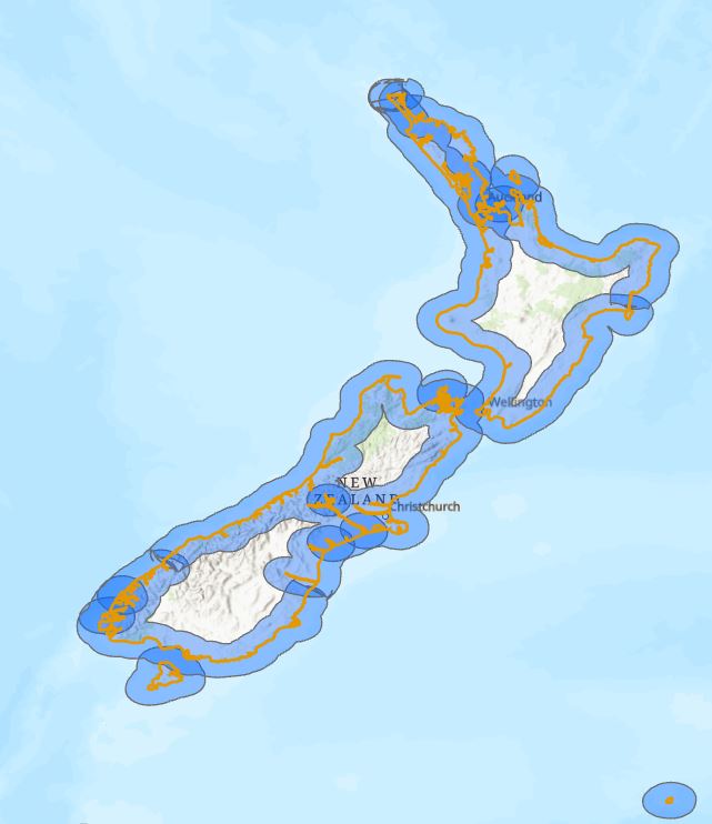
If I set up a 20 nm buffer around the ecoregions, here’s what I get (zoomed in to X to show the issue):
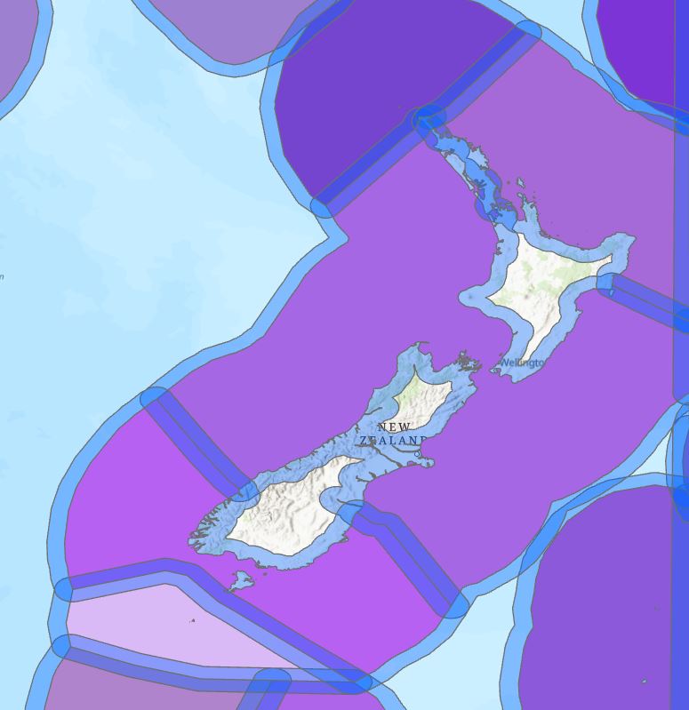
The blue areas are the buffers around each ecoregion. This layer nicely covers the 20 nm inland areas but the problem is that it also includes the areas that are mid-Tasman Sea. And since each ecoregion has a neighbouring region, we get overlapping buffers at those boundaries between ecoregions. Buffering gets me part of the way there but not close enough – I’m having trouble seeing what I can do with this output.
Buffers are created around each polygon feature, that’s creating more work here, soooo, what if I convert my polygons to lines and then buffer the lines? I used Feature to Line here which converts my polygons edges to lines up while also retaining all the original attributes:
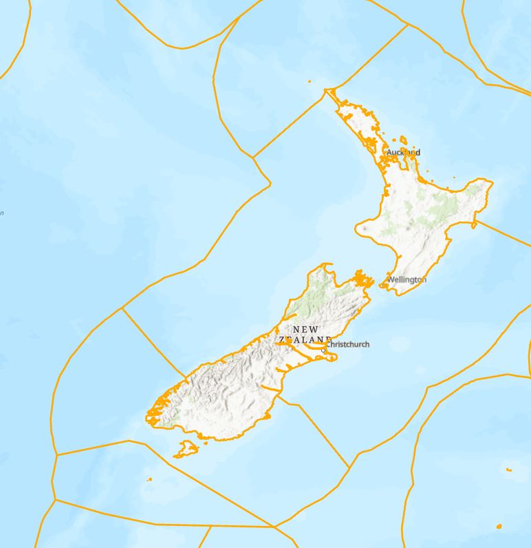
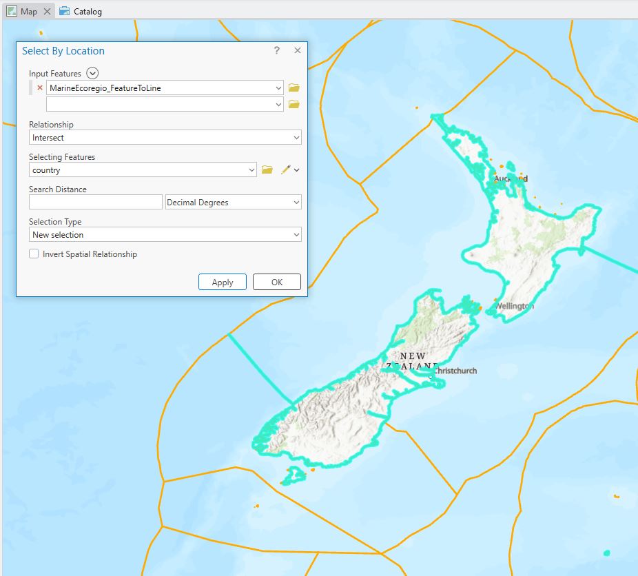
From this I’d like to just be able to have the lines that coincide with the edge that meets the shoreline. I could go through and manually remove the ones I don’t want – but that’s going to be a painstaking process and I’ve got a life to live. If you recall from previous images, the ecoregions go right up to shorelines, so if I had a layer of country boundaries, I could use that to select features that intersect with that boundary. After looking at a few, I used on that looked like it had the right level of detail and then did a select by location to find those features right on the border:
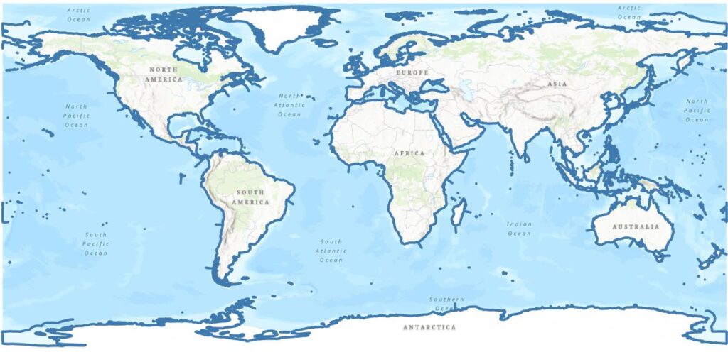
Nice, but see that I’m also getting some of the ecoregion boundaries, but I’m pretty happy with this. Exporting to a new layer gets me one step closer – here’s the global map:
Not bad, but the continents look a bit spikey. How can I find them and delete them? Are they all the same length (no)? If they are I could select all the ones with the same length and delete. Looking at the table, they’re not all the same length and there are some islands with shorter lengths. With one selected I did note an interesting thing in the table:

Each border line is actually two – one for each side of the neigbours. Their Shape_Lengths are the same but their ECOREGIONs are different. This makes sense when I think about it, but how can I systematically find them all and delete them? The Find Identical tool works a treat here. It will find records with identical values for an attribute and package them up nicely in a table for me:
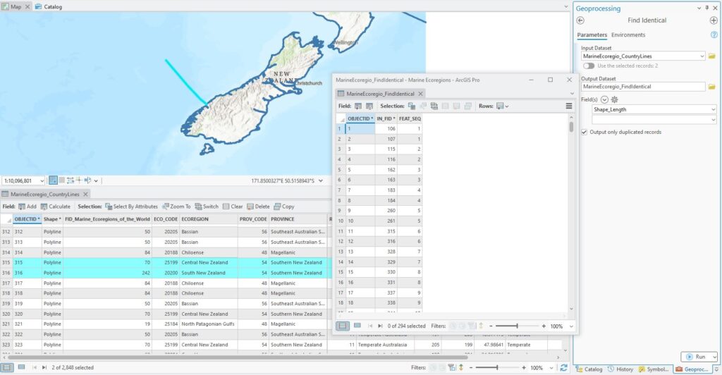
It’s a simple table – a row for each set of records grouped by FEAT_SEQ (the sequence in which they were found) and the IN_FID (the OBJECTID) of the original features. The records I have selected in the attribute table have OBJECTIDs of 315 and 316. In the Find Identical table, they are captured in records 11 and 12. If I now use a table join to link the Find Identical table to the line layer, that will help me find those records Where records have been matched, there will be a value for IN_FID while unmatched records get a Null value so I can use that in a Select by Attribute:
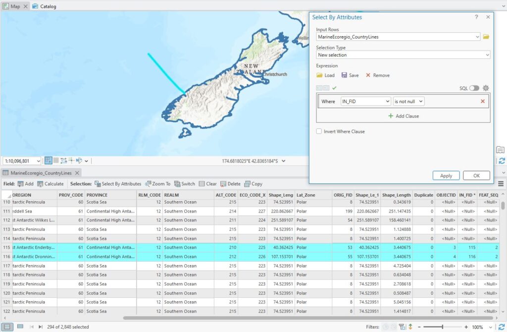
Sometimes using “is null” and “is not null” in the query can be really handy.
Duly selected, duly deleted. Now what I have left in this layer is the inland lines of all the ecoregions. Upon reflection, all I’ve done here is create a new global coastline…BUT, to salvage my self respect, the difference is that this coastline is broken up into the correct ecoregions, so life isn’t so worthless after all (Ed. that’s a bit dire…maybe you just need to get some fresh air.) Right – we’re edging (excuse the pun) ever closer to what we need.
Next I’ll run Buffer on my line layer with a 20 nm distance. Astute viewers will realised that I have an option to dissolve all the buffers into one feature or not. I don’t want to dissolve in this case as I’ll lose the information about individual ecoregions that I really need here. Here’s what I got:
Almost there – I’ve got the buffer zone on each side of the orange shoreline but I’m only interested in the inland areas. Using the MEOW layer with the Erase tool lets me remove the off shore areas:

Ever so close now – I next need to tidy up those overlapping buffer zone. When looking at the features and the table, I noted that some areas shared the same ECO_CODE. I’ll label them so you can see what I mean (also turned on MEOW and labelled each polygon with its ECO_CODE:
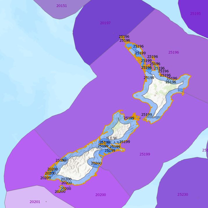
See how they match? Knowing this, I’m going to run the Dissolve tool on the ECO_CODE attribute and Bob should then be my proverbial uncle:
Feeling pretty good about this – it’s not perfect, mainly because at each overlap, Dissolve has to choose one feature’s buffer over another, so they don’t line up perfectlyl, but on a global scale I think I can live with this.
BUT…we’re not quite finished. To finish the job I need to combine these inland areas with the existing ecoregions, thereby extending them further inland. This was done in three steps: Merge > Table Join > Export Features, the end result being a new version of MEOW that includes the inland areas. Then we can start to see how well they’ll capture the observations with no ecoregion or major fishing area values (my 200,000+ observations):
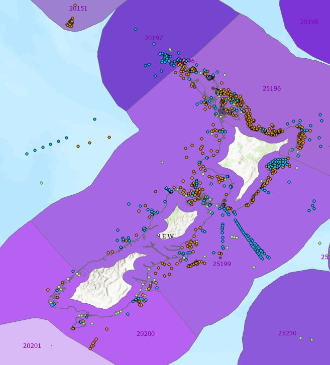
As a summary, here’s how this improved things with our existing global data:
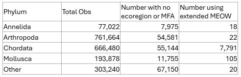
The remaining uncategorised observations are those around the large inland water bodies and/or further inshore than 20 nm. Chad tells me we can live with those, so I think my job here is done…for now at least. We’re expecting another tranche of data so I’ll get to do those extractions alllll ovvveeeer agaiiiiin!
As I alluded to at the start, this was one of those classic situations where at first it sounded like this would be a simple task, but when push came to shove (Ed. who was shoving whom here?), things got a lot more complicated than expected. Nonetheless, I think we got a pretty good outcome here using a range of classic vector tools.
Now if you’ll excuse me I feel like I’d like to get as far inland as I possibly can at the moment. (Fun fact, in NZ that’s roughly Cromwell at ~119 km inland.)
C
Postscript: as often happens, I finished writing this and, as I was walking home, came up with at least two other ways to do this, both of which might be far simpler and faster…so stay tuned (assuming you’ve made it this far).