
The Cat(fish)’s MEOW
We look at mapping observations of different marine species globally.
It’s been said that we know more about the surface of the moon than we do about our own Earth-bound oceans. I suspect that’s true. The amount of data available once we step off the land and into the briny is quite limited compared to terrestrial data. So we were pleased as punch when marine scientist Chad got in touch recently with some spatial interests. In this post I’ll cover the mapping side of what we did from start to finish and some useful things I learned along the way.
With a dataset of over 2 million points in his dataset of marine animal observations, Chad would like to know which marine ecoregion (from the Marine Ecoregions of the World (MEOW)) each point is in as well as which major fishing area it’s in (from the UN Food and Agriculture Organization (FAO)).
We started, as we often do, with an Excel spreadsheet of data. Five sheets broken down by phyla: Annelida, Arthropoda, Chordata, Mollusca, and Other, extracted from the Ocean Biodiversity Information System. Being of the spatial persuasion, the first thing I’m looking for in these data is something I can use to map the points:

See it? It helps if you’ve got a sense of what coordinates from different systems look like as we need to know which coordinate system they are in for mapping. Happily, the decimalLatitude and decimalLongitude columns look like they are coordinates in decimal degrees, and most likely in WGS84, so there’s my opportunity to get the points on the map.
Before I go too deeply into mapping I’ve got some decisions to make around how to handle these data. Each sheet has its own set of phylum data, with a minimum number of records in Annelida (77,022) and a maximum in Arthropoda (761,664). Do I want to keep these sheets separate or bring them all together into one table? Pluses and minuses to both but this time I chose to leave them as they are, so as to maintain the structure of the data Chad sent (which I may regret later…).
My next step is to get some points on the map. When each sheet is added to the map (using Add Data) they end up as standalone tables in my Contents pane:

As we’ve seen many times before, I can then use Right-click > Create Points from Table > XY Table to Point. (Alternatively, you can do this from Add Data > Points from Table > XY Table to Point). Et voila! Something to work with:
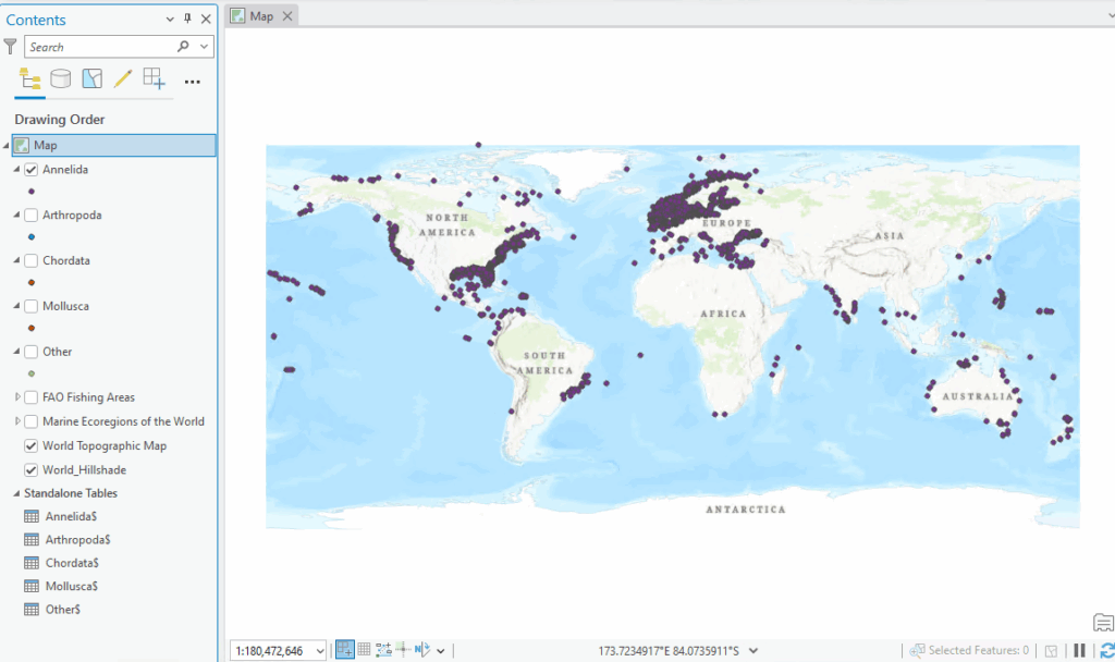
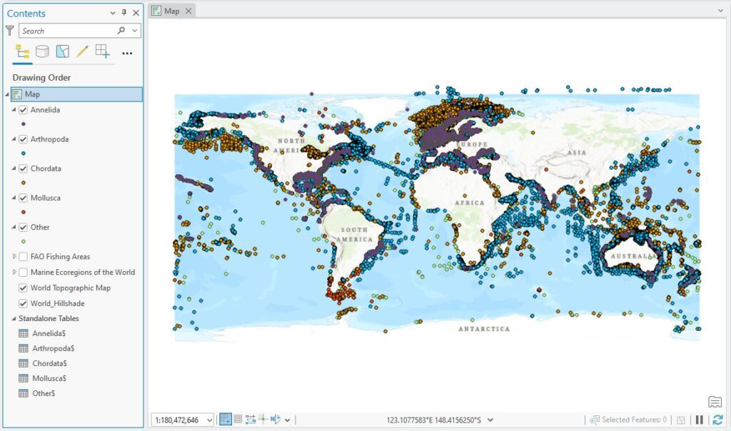
Things get busy when the other layers are turned on – we’ve got over 2 million points on the map now:
Busy busy. Let’s have a quick look at the data we’re going to be extracting from. First, MEOW:
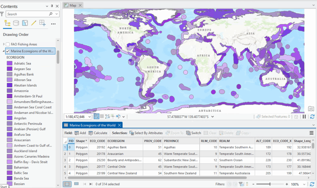
314 different marine ecoregions. Chad has asked if I can extract the ECO_CODE, ECOREGION, RLM_CODE and REALM attributes from this layer to each point. We can anticipate that not all of the points are going to sit in one of the ecoregions, and that’s why we have the FAO layer – to fill in any gaps:
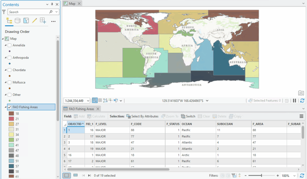
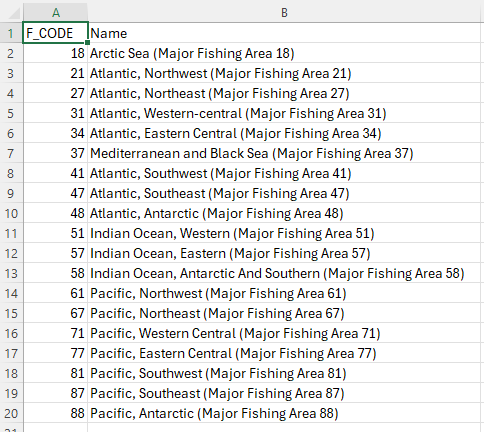
(I’m not sure that fish really respect those nice rectangular areas, but what do I know?) In this layer I’m mainly interested in the F_CODE attribute, which identifies each major fishing area. In an email, Chad sent me the names that go with each F_CODE which I then added to a CSV file for use later:
One of the things we noticed when getting familiar with the data was that neither of these datasets cover major inland water bodies, like the North American Great Lakes, but that’s just how it goes. Unfortunately, a not insignificant number of observations come from there but Chad tells me he’s mainly interested in salt water species so it’s not a big concern.
Now I’m poised to extract some data starting with MEOW. First, I’ve added four new attributes to each point layer’s table: ECO_CODE, ECOEGION, RLM_CODE and REALM. Once I’ve added the MEOW data I’ll populate each using Calculate Field.
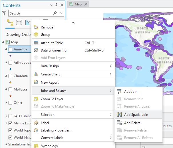
To extract the data I could run an Intersect spatial join, but any points that aren’t in an ecoregion won’t be returned, so an Identity would be better. A problem with both of these is that they create a new output layer. Plus, when using Identity I can only extract from one layer at a time, meaning I’d end up with an additional ten layers in my database. So to keep things simple, I’m going to set this up as a temporary spatial join from the Joins and Relates menu > Add Spatial Join instead:
This lets me set up a join based on where the two layers intersect:
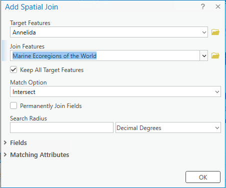
Ticking “Keep All Target Features” means I won’t lose any records. This temporarily adds in the attributes from MEOW to each record. Using Calculate Field I then copy the contents of each joined field to my new attributes :
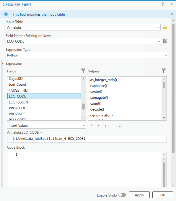
The ECO_CODE from the spatial join attributes is available under the Fields window and is shown as !Annelida_AddSpatialJoin_4.ECO_CODE! when added to the “Annelida.ECO_CODE =” window. When I run this calculation for each of the new attributes and then remove the spatial join, they now become a full-time, member in good standing of my point layer:
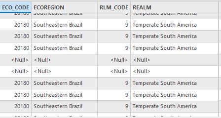
If a point doesn’t intersect with a MEOW polygon, it gets a Null in the table, as we can see with two records above.
You’ll recall that I need to do this with the FAO layer next to fill in as many of the MEOW gaps as we can. We follow the same steps to add those data in but the only thing I can really extract is the F_CODE. I need to join my CSV table to each point layer to link the F_CODE to a named fishing area. So add in some new attributes, add the major fishing area CSV table to my map, do the spatial joins and Calculate Fields (two joins, two calculations; one each for the FAO layer and for the CSV table). This brings everything together into one layer:
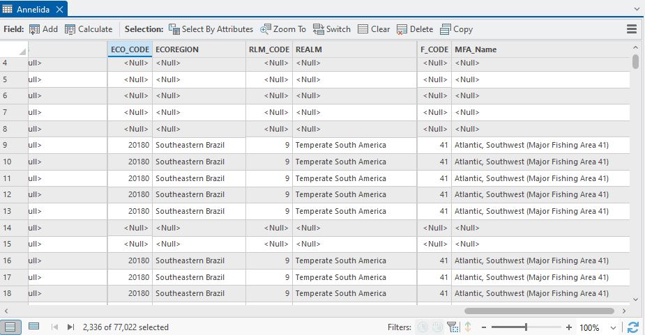
When looking over these results, adding the FAO data hasn’t made a huge difference, which is mostly down to those large inland water bodies. The selected records below are ones where it did actually fill in a MEOW gap, but, for example, out of my 77,022 Annelida records, it’s only filled in the gaps for 2,336.
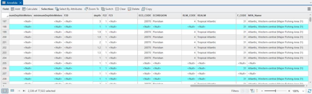
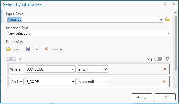
Alas, that’s the way that cookie crumbles, or…the kina crawls, or the sea snake swims, pick your cliche (I found these using a Select by Attribute where ECO_CODE is null AND F_CODE is not null, by the way).
As a final piece to this reasonably straightforward puzzle, Chad needs a copy of these results. I did this in two ways: an updated Excel spreadsheet and a webmap.
When exporting the spreadsheet using Table to Excel, I discovered a nice thing. I was anticipating that I’d have to run this tool five times and then combine all into one spreadsheet, but as you can see below, the tool allows you to add multiple table and they all end up in one output:
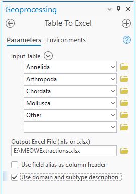
A nice little time saver that I wasn’t aware of before.
Lastly, I set up a webmap so that Chad could have a look at the data for himself. Have a look and see for yourself.
There was a nice combination of fundamental GIS-y sorts of things in this: adding data from a spreadsheet, spatial and table joins, adding attributes, calculating fields. As usual at the end of work like this (and even while you’re doing it) it’s helpful to think about how things could have been done differently. The biggest issue was the one at the start: keep the data separate or merge them into one table? There were times when I was doing the same thing over and over that I thought, surely there’s got to be a better way. It could have saved myself a lot of redundancy. The flip side is that those fewer steps would have taken longer as they had more data to crunch through, plus I think I would have wanted to separate them back out into their phyla before sending to Chad. Thinking about it now, I don’t think it would have made a major difference but reflection on workflows is always a good thing.
The other thing to reflect on was Identity versus a temporary spatial join/calculate field. With Identity I don’t need to do the Calculate Field step but I end up with lots of intermediate layers that I need to either ignore or actively delete. With the temporary spatial joins, yeah, I had more additional steps, but in the end have fewer data management issues. I could have set up a model to do this and if we end up repeating this with different input data, that effort might be worthwhile.
These are all good things to think about when figuring out your workflow.
All in all, a fun(ish) morning(ish) was spent working on this. It’s great to see some oceanic, off-shore applications with GIS and I’d look forward to doing a bit more of this wet work.
C